Results & discussion

The original training notebook preserves the optimizer’s termination message, a plot of training and test cost, and four final training predictions. These are the primary results presented here. No model has been retrained to replace them.

The recorded training run

Optimization terminated successfully.
         Current function value: 0.002864
         Iterations: 80
         Function evaluations: 82
         Gradient evaluations: 82

The run used the 2–3–1 architecture, $\lambda=0.0001$ , BFGS, and a maximum of 200 iterations. It terminated successfully after 80 iterations, using 82 function evaluations and 82 gradient evaluations.

“Successfully” is the optimizer’s termination status. It does not establish that the model found a global optimum or that it generalizes to new students.

The final objective, 0.002864, includes both normalized data error and the L2 penalty. It is neither an accuracy percentage nor an error measured directly in test-score points.

The original learning curve

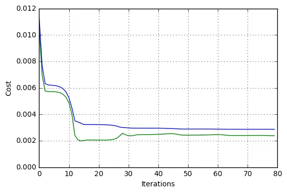
Original saved plot of training and test regularized cost over the optimizer iterations. Both fall sharply at the beginning and settle at lower values. — Figure 6. The original image embedded in training.ipynb, extracted without rerunning the notebook. The plotting code draws training cost first, then test cost; the original figure has no legend.

The code plots T.cost_list followed by T.test_cost_list. The image records a rapid initial decrease and lower costs later in the run. It illustrates the trajectory of this optimization, but the underlying arrays were not serialized as notebook output.

The chart’s horizontal axis is labeled “Iterations.” More precisely, the plotted positions are zero-based indices into the callback history. The vertical axis includes regularization on both splits.

Because the original figure is the surviving record, this site does not invent per-iteration values, add synthetic tooltips, or infer precise test metrics by reading pixels. The different input scales are also a material limitation when interpreting the test curve.

Predictions on the training examples

The notebook evaluates NN.forward(train_x) after training. Multiplying those saved normalized values by 100 gives:

Table 3. Saved training predictions, converted from 0–1 to points out of 100.
Example	Observed	Predicted	Error (points)
1	75.00	75.13	0.13
2	82.00	80.02	-1.98
3	93.00	83.65	-9.35
4	70.00	80.70	10.70

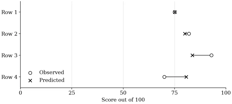
Observed scores shown as open circles and predicted scores shown as crosses, with a connecting line for each residual. Row 1: 75 versus 75.13. Row 2: 82 versus 80.02. Row 3: 93 versus 83.65. Row 4: 70 versus 80.70. — Figure 7. A new visualization of the four archived training predictions. Connecting lines show each residual; exact values are in Table 3.

The first example is close to its target. The largest absolute discrepancy is the fourth example: a prediction near 80.70 for a target of 70. The third example is underestimated by about 9.35 points. Looking at individual residuals makes the result more informative than a small normalized loss alone.

The console helper in the Python file converts each score to an integer before printing it, which truncates the fractional part. Table 3 uses the more precise notebook output instead.

Measurements derived from the archive

The following measurements are calculated for this site from the four saved predictions. They were not reported as these metrics in the original notebook.

Mean absolute error: 5.5396 score points.
Root mean squared error: 7.1734 score points.
Mean squared error: 51.4574 squared score points.
Mean half-squared error, normalized: 0.002572868, excluding regularization.

For score predictions $\widehat s_i$ and observed scores $s_i$ :

\begin{aligned} \operatorname{MAE} &= \frac{1}{m}\sum_{i=1}^{m} \lvert\widehat s_i-s_i\rvert,\\[0.75em] \operatorname{RMSE} &= \sqrt{\frac{1}{m}\sum_{i=1}^{m} (\widehat s_i-s_i)^2}. \end{aligned}

All of these are training-set measurements. The notebook does not preserve final test predictions, so a test MAE or RMSE cannot be calculated from the saved numerical output.

The normalized data term is approximately 0.002573. Subtracting it from the rounded reported objective suggests a weight penalty of approximately 0.000291. That difference is approximate because both the printed objective and the saved predictions have limited precision.

What worked

The forward pass was operational. The implementation mapped a batch of two-feature inputs to one prediction per row.
The backpropagation calculation had an independent check. Analytic and numerical gradient vectors matched at the displayed precision.
The optimizer consumed the supplied gradients. BFGS reported convergence within the specified iteration budget.
The project connected theory to executable code. Matrix shapes, the chain rule, regularization, and optimization all appeared in one small program that can be inspected in full.

These are concrete achievements of a first implementation. The network’s educational value comes from making each part explicit.

Limitations and lessons

Eight examples are not enough to support a general claim about student performance. There is no documented sampling procedure, repeated evaluation, uncertainty estimate, or comparison with a baseline such as a constant predictor or linear regression.

The preprocessing changes between splits. Training and test inputs are normalized independently. A future evaluation should fit normalization on training data and reuse it unchanged.

Regularization does not prove the absence of overfitting. The original conclusion says the regularization parameter prevented overfitting and preserved a model of the real world. A single run and the saved curve do not establish either claim. A regularization sweep or an unregularized comparison is not included in the archive.

Reproducibility is incomplete. There is no saved random seed, initial parameter vector, final weights, or full dependency lockfile. The curve’s values were saved as an image, not a numerical history.

The model has deliberate constraints. Nine weights, no biases, and sigmoid activations keep the exercise manageable. The sigmoid output bounds the score and can have small gradients in saturated regions.

An optimizer success message is not a validation result. It describes numerical termination on the chosen objective. It says nothing by itself about causal interpretation, out-of-sample error, or suitability for decisions about students.

What a follow-up study would add

A stronger follow-up would keep the original as a historical reference and run a separately labeled experiment: use a documented dataset, store a shared training-derived input scale, fix and report seeds, preserve weights and histories, compare simple baselines, and evaluate on untouched data. Multiple runs would show how sensitive the result is to initialization.

Those experiments are not part of the 2017 archive. The enduring finding here is the successful construction and inspection of a complete learning pipeline—and a clearer understanding of what is required to evaluate one.

Source: download the original training notebook. All derived measurements on this page are computed from its saved prediction array when this site is built.