Problem & foundations

The starting point was a small, concrete question: given the hours a student slept and studied before a test, estimate their score. A small example made it possible to work through every matrix operation and derivative.

A supervised regression problem

Each example pairs two inputs with one known output. The inputs are hours slept and hours studied; the target is a test score out of 100. A network receives those examples and adjusts its weights to reduce the difference between its predictions and the known scores.

This is supervised learning because the training examples include the desired answers. It is regression because the answer is a numerical quantity, rather than a category such as pass or fail.

\begin{aligned} \mathbf{x}_i &= [\,x_{i1},\ x_{i2}\,],\\[0.5em] y_i &= \frac{s_i}{100}. \end{aligned}

Here the two components of $\mathbf{x}_i$ are the input features after scaling, in sleep–study order. The raw score is $s_i$ ; the normalized target is $y_i$ . The data chapter spells out the input scaling.

The original introduction illustrates the task with three observations in raw hours and score points: $(3,5)\mapsto75$ , $(5,1)\mapsto82$ , and $(10,2)\mapsto93$ . The implementation adds a fourth training observation and four test observations. The data chapter lists the complete dataset.

The source header calls this an SAT-score example, but the code and manual actually use scores out of 100. This account follows the implemented scale.

Where this sits in machine learning

The manual introduces three learning settings:

Supervised learning: learn from examples containing both inputs and target outputs. This project belongs here.
Unsupervised learning: find structure in inputs without supplied target labels.
Reinforcement learning: learn actions through interaction and rewards.

The network does not receive a rule saying that a certain number of hours should produce a certain score. Its trainable weights define a family of functions, and optimization searches that family for a function that fits the supplied examples.

Learning a mapping is different from establishing a cause. These examples cannot establish the effect of sleeping or studying on test scores. Their role here is to exercise a learning algorithm, and the archive provides no description of how they were collected.

From a biological analogy to an artificial neuron

The manual uses a biological neuron as an intuition for receiving, combining, and transmitting signals. It is an analogy, not a biological model of the brain.

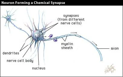
Original illustration of a biological neuron, showing dendrites, the cell body, and an axon. — Figure 2. The biological analogy used in the original introduction.

A computational neuron combines numerical inputs using a weighted sum. A positive weight increases the contribution of a positive input; a negative weight decreases it. The neuron then applies an activation function. In the following expression, $d$ is the number of inputs, $k$ selects an input, and $j$ selects a neuron.

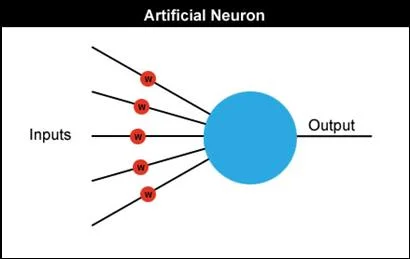
\begin{aligned} z_j &= \sum_{k=1}^{d} x_k w_{kj},\\[0.5em] a_j &= \sigma(z_j). \end{aligned}

Original artificial-neuron diagram: weighted inputs feed a summation and an activation function to produce an output. — Figure 3. Inputs, weights, summation, and activation in the original manual.

Many formulations add a bias $b_j$ to the weighted sum. This implementation has no bias parameters, so the equations on this site omit them too. That makes the parameter count small and changes the functions the model can represent.

Why the activation matters

Without nonlinear activations, stacking matrix multiplications would still produce a linear mapping. The sigmoid introduces a nonlinear transformation:

\sigma(z)=\frac{1}{1+e^{-z}}

Its output lies between zero and one, which matches the normalized target scores. A prediction of $0.82$ becomes 82 points after multiplying by 100. The output is a normalized score estimate; it is not a probability that a student earns a particular score.

The sigmoid is smooth and differentiable, making it possible to calculate how the loss changes as each weight changes. It can also saturate near either end of its range, where its derivative becomes small. The architecture chapter makes this behavior explicit.

Prediction, error, and learning

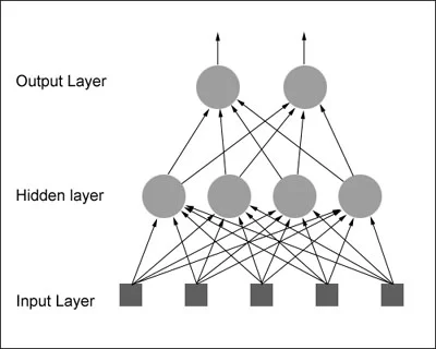
Original diagram illustrating an artificial neural network model and its learning process. — Figure 4. The original model illustration. The executable network is specified precisely in the next chapters.

The training loop ties three ideas together:

Predict: run inputs forward through the current network.
Measure: compare predictions with targets using a loss function.
Adjust: compute gradients and let an optimizer update the weights.

The original introduction writes the error as a sum of half-squared differences. The final implementation averages that data error and adds a penalty on large weights. Those details matter when interpreting the small objective value reported by the optimizer.

The central learning outcome was understanding that connection: a prediction is built from matrix operations, the loss measures its error, and the chain rule links that error back to every weight.

A note on the original terminology

This account retains the original diagrams and purpose while using corrected terminology. A network with many hidden layers is a deep neural network; it is not automatically a deep belief network. Likewise, learned weights are parameters, while choices such as layer sizes and regularization strength are hyperparameters. The original architecture table reverses those definitions.

Source: original introduction notebook and Python implementation.